Characterizing Extrachromosomal DNA Regions with Graph Neural Networks
Background and Research Goals
Extrachromosomal DNA (ecDNA) are amplified fragments of the genome that exist away from the chromosomes and has shown to be found in aggressive forms of cancer. From a genomic perspective, ecDNA regions should be identifiable from the presence of frequently occurring, repeated strings of base pairs. However, homogeneously staining regions (HSRs), which lie on the chromosome itself, are also repeated DNA sequences but are benign in comparison to ecDNA. This complicates the problem of identifying ecDNA because there exist two types of repeated genomic sequences that sequentially, appear largely the same.
Prior studies [7] have shown that ecDNA interacts more evenly with DNA regions on other chromosomes whereas HSRs tend to favor some over others. Mathematically, ecDNA have higher trans-to-cis contacting ratios than HSRs, meaning that the chromosomal interactions of ecDNA tend to be more with other chromosomes whereas those of HSRs tend to be higher in their host chromosomes. We aim to characterize ecDNA regions, while also being able distinguish them from HSRs, by capturing the inherent graphical structure of genomic interactions by utilizing graph-based methods like node2vec [2] and GraphSAGE [3].


Figure 1: ecDNA (left) and HSR (right) 3d Structure
Data: Hi-C Matrices and RNA-seq Reads
We align RNA sequencing reads from the GBM39 cell line to the hg38 (human) reference genome for both ecDNA and HSR. The genome is divided into 5000 base pair (bp) segments, and each mapped read is assigned to one of these regions. This process is repeated with gene annotation data, assigning genes to every genomic region in which they are present, allowing a gene to be counted in multiple regions. As a result, we obtain read and gene counts for each genomic region for both ecDNA and HSR. Our read counts serve as a proxy for gene expression. Next, we narrow our focus to the loci captured by the Hi-C matrices and adjust our dataset to match these regions.
Hi-C matrices contain values corresponding to the frequency of interactions between two genomic regions [8]. Our Hi-C data captures genomic regions on chromosome 7 between loci chr7:54750000-56005000. We have two Hi-C matrices, each a 251x251 adjacency matrix, for both ecDNA and HSR. Since all Hi-C values are non-zero, arranging this information directly into a graph results in two almost identical complete graphs, severely roadblocking our graph-learning tasks. To address this, we follow a thresholding protocol using the top 25% of interactions [1]. We bin each region by Euclidean distance, subtract the 75th percentile distance of the bins from each region’s Hi-C value, and discard all negative values. The remaining edges are then converted to 1s, resulting in a binarized adjacency matrix with 1s for significant genomic region interactions and 0s for others. This aligned sequencing data and pruned Hi-C matrix are the data that will be used throughout our analysis, modeling, and discussion.
Interaction Graphs
Check out our Interactive Graph Visualization .
Interactions graphs simplify visualizing all 251 genomic regions for both ecDNA and HSR. For ease of visualization, we arbitrarily selected a genomic region to demonstrate the differences between ecDNA and HSR at the same loci.


Figure 2: ecDNA interaction graph (left) and HSR interactions graph (right) with same regions selected
Methods
Clustering
We develop a pipeline as below to cluster our data. We take our ecDNA interaction graph, as defined above; apply node2vec [2] on it, giving us 16-dimensional vectors for each node; append the read counts and gene counts to the embeddings; reduce the data to 2 dimensions using PCA; and lastly cluster the data using DBSCAN. We then repeat the process on the HSR graph.
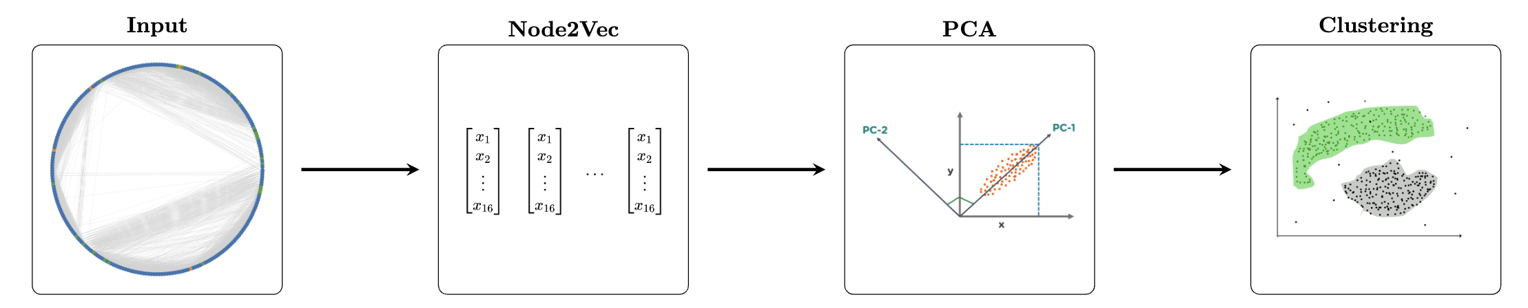
Figure 3: Clustering Pipeline
In more detail, node2vec [2] is a technique for learning continuous feature representations for nodes in a graph, preserving both local and global structural properties. It achieves this by simulating biased random walks on the graph, generating sequences of nodes similar to sentences from a natural language processing standpoint. These sequences are then used to train a Skip-Gram model, akin to Word2Vec, to learn embeddings that capture relationships between nodes. On a high level, we want nodes that are similar, in terms of both homophily and structural equivalance, to lie close together in the embeddings space. It is a powerful model to learn information-rich embeddings for our nodes. DBSCAN allows us to find an unspecified number of clusters because we did not have a pre-specified amount of classes that we were looking for.
After reducing the dimensionality of our node embeddings, we applied DBSCAN. DBSCAN is a clustering algorithm that groups closely packed points based on two parameters: epsilon (ε), the maximum distance between points to be considered neighbors, and minPts, the minimum number of points to form a dense cluster. It identifies core, border, and noise points, allowing it to detect clusters of arbitrary shapes and isolate outliers without needing to predefine the number of clusters. Since we did not have a specific number of clusters to classify into beforehand, this characteristic was the deciding factor in face of K-Means approaches, where we pre-define the number of classes.
Classification
GraphSAGE is an inductive graph learning algorithm that simultaneously learns the graphical structure of the neighborhood of a node and the distribution of their features to create aggregated embeddings for each node in the training set of a graph [3]. For each node in the training set, denoted as the target node in the figure below, GraphSAGE samples its neighbors and aggregates their node features to update node embeddings. The vector containing the aggregated information of the neighbors is concatenated to the current state of the embedding for the target node. The final set of node embeddings contain information about the node features of its neighbors and the structure of the graph around it.

Figure 4: GraphSAGE Algorithm Visualization Link to Source
GraphSAGE is useful for our classification problem due to differences in genomic interaction and genetic expression between HSR and ecDNA. In terms of genomic interaction, ecDNA has a circular structure [5], whereas HSR does not, allowing regions within ecDNA to uniquely interact. In terms of genetic expression, ecDNA is more expressive than HSR. Its existence off of the chromosome amplifies the genes it contains. Genomic interaction is represented by the edges in our graph, and expression is captured in the graph through the RNA-seq read count feature of the node vector. Notable differences in interactions and expression, captured by the structure and node features of the graph, naturally lead to the use of GraphSAGE for the classification task.
We trained GraphSAGE on a graph containing both the ecDNA and HSR portions, with each being a disjoint subgraph of a larger graph. Our model followed an encoder decoder paradigm. The encoder consisted of two GraphSAGE layers that generated 16-dimensional embeddings for each node. The decoder consisted of two linear fully connected layers with ReLU activation, reducing the dimensionality to a 2 dimensional output layer. Softmax was applied to the output layer for classification, and Cross Entropy loss was used to evaluate predictions and train the model.

Figure 5: Classification Pipeline
Results
Clustering Results
These are the results of PCA and subsequent clustering for ecDNA (left) and HSR (right).
.png)

Figure 6: ecDNA (left) and HSR (right) PCA clusters
We visualized these clusters by overlaying their locations on top of the heatmap of the corresponding HI-C matrix. We also attached a gene track under each of the plots to visualize which genes were present within our loci range. It allows us to compare whether clusters match up with the presence of genes.
.png)
.png)
Figure 7: ecDNA (left) and HSR (right) HI-C heatmap with clusters and gene track
After computing these clusters, we checked if these clusters created significant differences in terms of multiple graph properties. Specifically, we applied a Mann-Whitney U-Test on all pairs clusters for each property that we were interested in. The following heatmap shows the p-values for each U-Test that we conducted. We defined significance at p < 0.05.
.png)
Figure 8: ecDNA U-Test P-Values
.png)
Figure 9: HSR U-Test P-Values
Classification Results
We trained our GraphSAGE classification model on the combined graph G, obtaining the results in the table below. We split the graph into train, validation, and test sets using masks with a split of 70%-15%-15%. The test metrics in the table display the results of predictions on both the validation and test sets. Early stopping [4] was implemented to capture the best performing model during training.
| Metric | Train | Test |
|---|---|---|
| Accuracy | 0.92308 | 0.81333 |
| Precision | 0.92327 | 0.82799 |
| Recall | 0.92294 | 0.82719 |
| F1 Score | 0.92304 | 0.82744 |
.png)
Figure 10: GraphSAGE Results Table (left) and Confusion Matrix (right)
Takeaways
Clustering
We defined three different types of clusters given our results - the sparse outliers, the dense core, and the more tightly clustered regions. We examined the nature of these three and came away with three conclusions:
-
Differences in ecDNA and HSR clusters suggest distinct sets of similarly behaving genes specific to each structure. We hypothesize that these differences in clusters from ecDNA and HSRs could come from their different 3d structures. Specifically, it tells us that in ecDNA, certain genomic regions are being brought together in new spatial neighborhoods, likely exposing different genes to regulatory elements like enhancers or promoters. Conversely, in HSRs, different clusters suggest a different structural pattern, which may be causing the regulation of an alternate set of genes
-
Less populous clusters within ecDNA reveal structurally related genes. The plot below shows how regions in the same cluster that correspond to genes are related in 3D space. For example, we can see two regions from Cluster 5 that correspond to genes NIPSNAP2 (blue) and ZNF713 (lime). Now from the figure on the right, we can see that these genes lie along a loop in 3d space. This gives us evidence toward the fact these genes may share regulatory elements like promoters or enhancers and be co-regulated/co-expressed in ecDNA.
.png)
.png)
Figure 11: Left: ecDNA Structure with Clusters 4 and 5 highlighted Right: Same as Left but specific genes highlighted
- Graphically, the two most populous clusters in ecDNA and HSR behave significantly differently. At the 5% significance level, the only two clusters that were significant in all of the graph properties we looked at were Cluster 1 (outliers) and Cluster 2 (dense core). These two clusters behave distinctly when it comes to HI-C interactions and gene/read counts.
Classification
Of the four metrics we used to evaluate GraphSAGE, accuracy and recall are the most critical for our problem. Recall is particularly important for our task due to the cancerous properties of ecDNA. Recall weights false negatives, which for our problem, means predicting HSR (a benign region) when the region is ecDNA (a cancerous region). Failing to diagnose a patient with cancer is far more harmful than diagnosing a non-cancer patient with cancer, the false positive case. Fortunately, our GraphSAGE is generating balanced predictions, as seen in the confusion matrix.
GraphSAGE performed well on both the train and test sets, but there is a notable discrepancy of about 0.1 in each metric between the two sets. This is likely due to the small size of our dataset. However, strong performance on the train set is a positive indicator that GraphSAGE was able to find patterns in the graph structure and node features differentiating ecDNA and HSR. Obtaining more cell samples on the GBM39 cell line can boost the robustness of our graph learning model. To further extend research on the classification task, GNNExplainer [6] can be attached to the GraphSAGE model to learn key predictive regions of the graph. These subgraphs can be matched to their 3D location, which could uncover key differences in structure between ecDNA and HSR.
We are extremely encouraged that our model was able reach over 80% accuracy with such a limited dataset given that we had only ~400 training points and used <0.1% of the human genome. It only goes to show the strength of a graph-based approach. We call for further work, with a broader range of data, to be done with GNNs in this context of this problem.
References
[1] Bigness, Jeremy, Xavier Loinaz, Shalin Patel, Erica Larschan, and Ritambhara Singh. 2022. “Integrating long-range regulatory interactions to predict gene expression using graph convolutional networks.” Journal of Computational Biology 29(5): 409–424 Link
[2] Grover, Aditya, and Jure Leskovec. 2016. “node2vec: Scalable Feature Learning for Networks.” Link
[3] Hamilton, William L., Rex Ying, and Jure Leskovec. 2018. “Inductive Representation Learning on Large Graphs.” Link
[4] Prechelt, Lutz. 2002. “Early stopping-but when?” In Neural Networks: Tricks of the trade. Springer: 55–69 Link
[5] Wu, Sihan, Kristen M Turner, Nam Nguyen, Ramya Raviram, Marcella Erb, Jennifer Santini, Jens Luebeck, Utkrisht Rajkumar, Yarui Diao, Bin Li et al. 2019. “Circular ecDNA promotes accessible chromatin and high oncogene expression.” Nature 575 (7784): 699–703 Link
[6] Ying, Rex, Dylan Bourgeois, Jiaxuan You, Marinka Zitnik, and Jure Leskovec. 2019. “GNNExplainer: Generating Explanations for Graph Neural Networks.” Link
[7] Chang, Lei, Yang Xie, Brett Taylor, Zhaoning Wang, Jiachen Sun, Ethan J Armand, Shreya Mishra, Jie Xu, Melodi Tastemel, Audrey Lie et al. 2024. “Droplet Hi-C enables scalable, single-cell profiling of chromatin architecture in heterogeneous tissues.” Link
[8] van Berkum NL, Williams L Imakaev M Gnirke A Mirny LA Dekker J Lander ES, Lieberman-Aiden E. 2010. “Hi-C: a method to study the three-dimensional architecture of genomes.” [Link][https://pmc.ncbi.nlm.nih.gov/articles/PMC3149993/]